Exareme

Exareme Dataflow Language

Extending Functionality

The system uses extensively the UDF extensions APIs of SQLite. SQLite supports the following UDF categories: Row functions take as input one or more columns from a row and produce one value. An example is the UPPER() function. Aggregate functions can be used to capture arbitrary aggregation functionality beyond the one predefined in SQL (i.e., SUM(), AVG(), etc.). Virtual table functions (also known as table functions in Postgresql and Oracle) are used to create virtual tables that can be used in a similar way with tables. The API offers both serial access via a cursor, and random access via an index. The SQLite engine is not aware of the table size allowing the input and output to be arbitrarily large. All UDFs are implemented in Python. Both Python and SQLite are not strictly typed. This enables the implementation of UDFs that have dynamic schemas based on their input data.

Dataflow Language

The dataflow language of Exareme (DFL) is based on SQL. We present some examples that use a subset of the TPC-H schema:

1. orders (o_orderkey, o_orderstatus, ...)
2. lineitem (l_orderkey, l_partkey, l_quantity, ...)
3. part (p_partkey, p_name, ...)

1. orders to 2 parts on hash(o_orderkey)
2. lineitem to 3 parts on hash(l_orderkey)
3. part to 2 parts on hash(p_partkey)

distributed create table lineitem_large as \\Distributed part
select * from lineitem where l_quantity > 20; \\Local part

In general, a query has two semantically different parts: distributed and local. The distributed part defines how the input table partitions are combined and how the output will be partitioned. The local part defines the SQL query that will be evaluated against all the combinations of the input (possibly, in parallel). In the example, the system will run the SQL query on every partition of table lineitem. Consequently, table lineitem_large will be created and partitioned into the same number of partitions as lineitem.

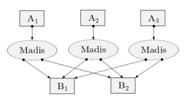
The output table can be partitioned based on specific columns. All the records with the same values on the specified columns will be on the same partition. For example, consider the following query were the user specifies the partition key (l_orderkey) and the number of output partitions(2).

distributed create table lineitemm_large to 2 on l_orderkey as
select * from lineitem where l_quantity > 20;

The execution plan produced by this query is shown in the figure below. The output of each query, is partitioned on column l_orderkey. Notice that all records with the same l_orderkey value must be unioned in order to produce the 2 partitions of table lineitem_large, creating the lattice after the queries are executed.

If more than one input tables are used, the table partitions are combined and the query is executed on each combination. The combination is either direct or a cartesian product, with the later being the default behavior. An example is the following query.

distributed create table lineitem_part as
select * from lineitem, part where l_partkey=p_partkey;

The system evaluates the query by combining all the partitions of lineitem with all the partitions of part. As a result, table lineitem_part will have 6 partitions (3 x 2). If tables lineitem and part have the same number of partitions, the combination can be a direct product. This is shown in the following query.

distributed create table lineitem_part as direct
select * from lineitem, part where l_partkey = p_partkey;

Notice that, in order the query to be a correct join, the tables lineitem and part must be partitioned on columns l_partkey and p_partkey respectively.

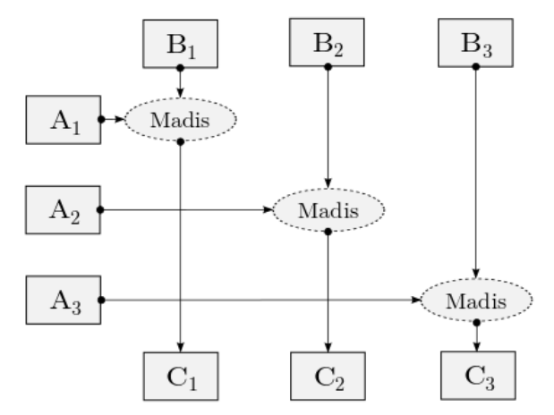
The local part of the query can be as complex as needed using the full expressivity of SQL enhanced with the extensions described above. Queries can be combined in order to express complex data flows. For example, a distributed hash join can be expressed as follows:

distributed create temporary table lineitem_p on l_partkey as
select * from lineitem;

distributed create temporary table part_p on p_partkey as
select * from part;

distributed create table lineitem_part as direct
select * from lineitem_p, part_p where l_partkey = p_partkey;

Tables lineitem_p and part_p are temporary and are destroyed after execution. Notice that in this example, the system must choose the same parallelism for tables lineitem_p and part_p in order to combined as a direct product. A MapReduce flow can be expressed as follows:

distributed create temporary table map on key as
select keyFunc(c1, c2, ...) as key, valueFunc(c1, c2, ...) as value from input;

distributed create table reduce as
select reduceFunc(value) from map group by key;

with, key(*), being a row function that returns the key of the row, and value(*) being a row function that produces the value. In the second query, the reduce(*) is a aggregate function that is applied on each group.